
|
Statistics
|

|
|
Many things we like to study actually vary according to the Normal distribution; that is, a graph of their distribution is symmetric and bell-shaped--that is, the peak is in the middle and the graph tapers off on both ends. For example, weight is a variable that is approximately Normal. Histograms can be used to illustrate a Normal distribution. In the histograms below, lists of \(100\) randomly generated weights of newborn babies (so a sample size of \(100\) out of the population) were created using the graphing calculator and then graphed. The population data has a mean of \(7.5\) pounds and a standard deviation of \(1.25\) pounds. Four different "random samples" were generated.
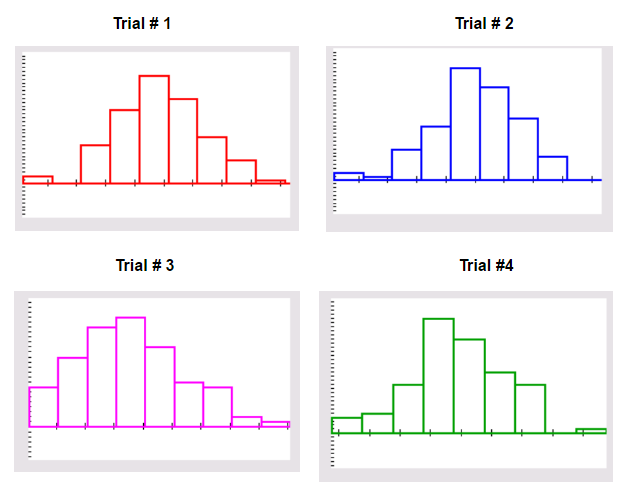
You can see that the four histograms vary slightly. If we were to repeat this activity with different samples of \(100\) newborns, the mean and standard deviation will be slightly different each time, as would the histograms, because our sample of \(100\) weights will contain different values. Instead of generating numerous samples and histograms, we can use a Normal distribution to give us measurable information regarding the population.
As you learned earlier, a sample is part of the entire population, so depending on the group selected as the sample, the data will differ slightly. However, if the sample size is large enough and the sample is randomly selected, the sample data will fairly accurately represent the population data.
When we study a sample of a population, we are usually interested in some measurable characteristic our subjects have, such as height, age, weight, etc. Many times the variable we measure behaves like the normal distribution, one of the most useful distributions in all of statistics.
Properties of the Normal Distribution:
- The mean, median and mode of the data set are approximately equal.
- The graph is symmetric about the mean.
- The area under the distribution = \(100\%\).
- The graph is bell shaped.
- The graph is continuous and will never intersect the x-axis.
Mean (\(\mu\)): Average of the data values
Standard Deviation (\(\sigma\)): Measure of variability of the data
Outlier: Any data value that is more than \(3\) standard deviations above or below the mean.
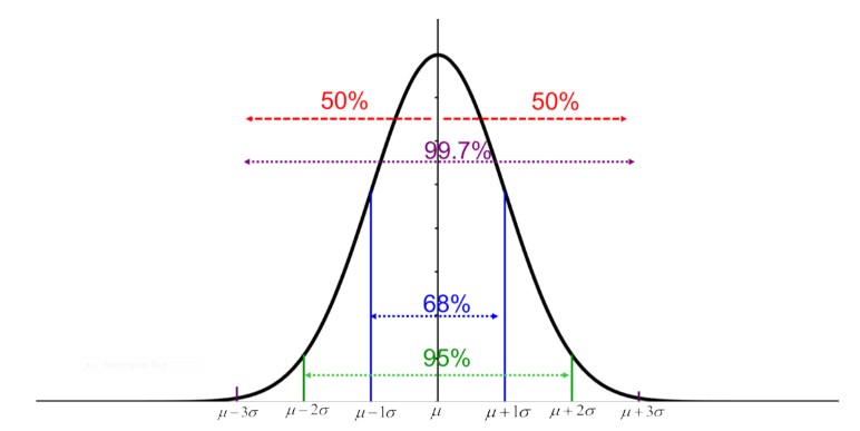
Explore the graph of the normal distribution below to find the percent of the curve that is shaded between \(1\), \(2\) and \(3\) standard deviations of the mean by moving the slider \(a\).
\(68-95-99.7\%\) Rule
\(68\%\) of all data values fall within \(1\) standard deviation of the mean.
\(95\%\) of all data values fall within \(2\) standard deviations of the mean.
\(99.7\%\) of all data values fall within \(3\) standard deviations of the mean.
Also,
\(50\%\) of all data lies above the mean and \(50\%\) of all data lies below the mean.
\(2.5\%\) of data is more than \(2\) standard deviations above the mean or more than \(2\) standard deviations below the mean.
Here is a breakdown of the normal distribution. Watch the video for a more thorough explanation.
|
|
Quick Check
The average monthly high temperatures in Chicago for \(2016\) are normally distributed with a mean of \(53^{\circ}\) F and a standard deviation of \(22^{\circ}\) F. Draw and label the normal distribution and answer the following questions.
a) What is the probability the average high temperature will be between \(31\) degrees and \(75\) degrees?
b) What is the probability the average high temperature will be between \(9\) degrees and \(97\) degrees?
c) What is the probability the average high temperature will be greater than \(97\) degrees?
d) What is the probability the average high temperature will be less than \(75\) degrees?
e) What is the probability the average high temperature will be between \(75\) degrees and \(97\) degrees?
f) What is the range for the middle \(99.7\%\) of average high temperatures?
g) The top \(16\%\) of average high temperatures are greater than what amount?
h) Give two high temperatures that would be considered outliers.
Quick Check Solutions
Example 1: Nationally, the average ACT composite score is \(20.8\) with a standard deviation of \(4.8\). Assume the data is approximately normally distributed.
a) What percent of the population scores between \(25.6\) and \(30.4\)?
b) What percent of the population scores below \(16\)?
c) What percent of the population scores between \(16\) and \(30.4\)?
Example 2: The standard deviation of a distribution describes how varied the measurements are. Because we must maintain an area of \(1\), or \(100\%\), under the curve, its shape will change for larger or smaller values of the standard deviation. How does changing the standard deviation affect the shape of the distribution? How does changing the mean affect the shape of the distribution? Move the sliders \(m\) for the mean and \(s\) for the standard deviation.
If the standard deviation is changed, the peak remains in the same location, but the graph flattens out for larger standard deviations and becomes more clustered about the mean for smaller standard deviations.
If the mean is changed, the peak remains the same height, and the spread of the data doesn’t change, but the peak will shift left or right depending on if the mean decreases or increases.
Standard Normal Distribution and z-score
Converting Percentiles to Statistics